Extracting measures with openSMILE ✲゚。.(✿╹◡╹)ノ☆.。₀:*゚✲*:₀。
While I didn’t get the opportunity to pursue my endeavors in speech processing just yet, I still gathered a bunch of resources over the course of my degree, which I thought I’d share, as speech processing tools can be a little niche. In this tutorial, we’ll see how to use the openSMILE toolkit for feature extraction, and later plot formants. :)
If you’re working on speech processing and analysis, it is likely that you’ve worked with some tools such as Praat, or Python libraries like librosa and Parselmouth. While these tools allow you to compute various measures that you can later explore and further analyse, and have imposed themselves as the standard in computational approaches, there’s also a growing interest for automatic feature extraction tools.
openSMILE is an extensive, open-source, toolkit for audio analysis, processing and classification, which is aimed for speech and music applications, introduced by F. Eyben et al in 2010. Specifically, it allows researchers to easily run feature extraction, either via CLI or its Python wrapper, opensmile-python. openSMILE is currently maintained by audEERING, a german company working on audio technology and the use of AI for various tasks (speech synthesis/text-to-speech…).
In this tutorial, we will see how to work with openSMILE’s Python wrapper to easily extract features from a short audio segment.
# needed librairies
import opensmile
import pandas as pd
import matplotlib.pyplot as plt
import seaborn as sns
extracting audio features ( ・_・)ノ
As of now, openSMILE supports three standard feature sets: ComParE 2016, which consists of more than 6,000 features, GeMAPS (Geneva Minimalistic Acoustic Parameter Set) and eGeMAPS, which come in variants. Those feature sets are configuration files which indicate the features that are to be extracted. While openSMILE offers the previously mentioned feature sets, it is also possible to create your own configuration file! Features can be extracted on two different levels:
- low-level descriptors (LDD)
- functionals
To get the full-list of feature sets openSMILE has:
for feature_set in opensmile.FeatureSet:
	print(str(feature_set))
FeatureSet.ComParE_2016
FeatureSet.GeMAPS
FeatureSet.GeMAPSv01b
FeatureSet.eGeMAPS
FeatureSet.eGeMAPSv01b
FeatureSet.eGeMAPSv02
FeatureSet.emobase
For more information on feature sets and a better understanding of the features (LLD and functionals) that are to be automatically extracted, you can read F. Eyben et al (2016).
file = "path/to/audio/file" # wav
# for context, I'm using a segment from an interview from CFPP
#(Corpus du Français Parler Parisien). speaker is Anita MUSSO (F, 46).
# path_to_audio = '../../aligned/aligner-corpus/Anita_MUSSO_F_46_11e-v2/Anita Musso_1056.942_1060.072.wav'
smile = opensmile.Smile(
		feature_set=opensmile.FeatureSet.GeMAPSv01b,
		feature_level=opensmile.FeatureLevel.LowLevelDescriptors
)
results = smile.process_file(file) # resulting DataFrame
results.head() # print first 5 rows
You can get feature names, feature levels and feature set used by a given Smile object with by using the feature_names property:
smile.feature_names # returns list of LLD for GeMAPSv01b
To get a better understanding of what’s in the results DataFrame, you can also use results.info().
<class 'pandas.core.frame.DataFrame'>
MultiIndex: 309 entries, ('../../aligned/aligner-corpus/Anita_MUSSO_F_46_11e-v2/Anita Musso_1056.942_1060.072.wav', Timedelta('0 days 00:00:00'), Timedelta('0 days 00:00:00.020000')) to ('../../aligned/aligner-corpus/Anita_MUSSO_F_46_11e-v2/Anita Musso_1056.942_1060.072.wav', Timedelta('0 days 00:00:03.080000'), Timedelta('0 days 00:00:03.130000'))
Data columns (total 18 columns):
 #   Column                       Non-Null Count  Dtype
---  ------                       --------------  -----
 0   Loudness_sma3                309 non-null    float32
 1   alphaRatio_sma3              309 non-null    float32
 2   hammarbergIndex_sma3         309 non-null    float32
 3   slope0-500_sma3              309 non-null    float32
 4   slope500-1500_sma3           309 non-null    float32
 5   F0semitoneFrom27.5Hz_sma3nz  309 non-null    float32
 6   jitterLocal_sma3nz           309 non-null    float32
 7   shimmerLocaldB_sma3nz        309 non-null    float32
 8   HNRdBACF_sma3nz              309 non-null    float32
 9   logRelF0-H1-H2_sma3nz        309 non-null    float32
 10  logRelF0-H1-A3_sma3nz        309 non-null    float32
 11  F1frequency_sma3nz           309 non-null    float32
 12  F1bandwidth_sma3nz           309 non-null    float32
 13  F1amplitudeLogRelF0_sma3nz   309 non-null    float32
 14  F2frequency_sma3nz           309 non-null    float32
 15  F2amplitudeLogRelF0_sma3nz   309 non-null    float32
 16  F3frequency_sma3nz           309 non-null    float32
 17  F3amplitudeLogRelF0_sma3nz   309 non-null    float32
dtypes: float32(18)
memory usage: 44.5+ KB
When looking at the output, you’ll notice we’re working with 3 indexes: file, start, and end, the last two being time dimensions. If those look weird, it’s because of the data type: time here is expressed as a “duration” (the corresponding pandas datatype is timedelta). Let’s convert them to seconds to make things easier. ‧₊˚❀༉‧₊˚.
results_pd.reset_index(inplace=True, level=['start', 'end'])
# convert timedelta to seconds
results_pd['start'] = results_pd['start'].dt.total_seconds()
results_pd['end'] = results_pd['end'].dt.total_seconds()
# display
results_pd.head()
The only index you’re working with now is file!
plotting formants (。・o・。)ノ
# extract center formant frequencies
df = pd.read_csv('path/to/extracted_features_pandas.csv')
centerformantfreqs = ['start','F1frequency_sma3nz',
                      'F2frequency_sma3nz', 'F3frequency_sma3nz']
formants = df[centerformantfreqs] # new dataframe with the columns we are interested in only
# resulting dataframe
formants.head()
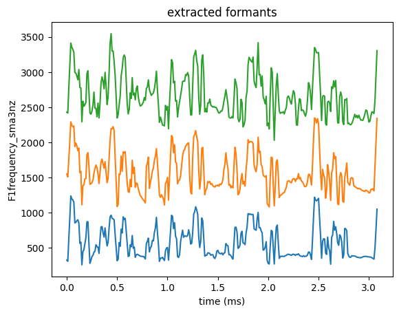
sns.lineplot(data=formants, x='start', y='F1frequency_sma3nz')
sns.lineplot(data=formants, x='start', y='F2frequency_sma3nz')
sns.lineplot(data=formants, x='start', y='F3frequency_sma3nz')
plt.xlabel('time (ms)')
plt.title('extracted formants')
plt.show()
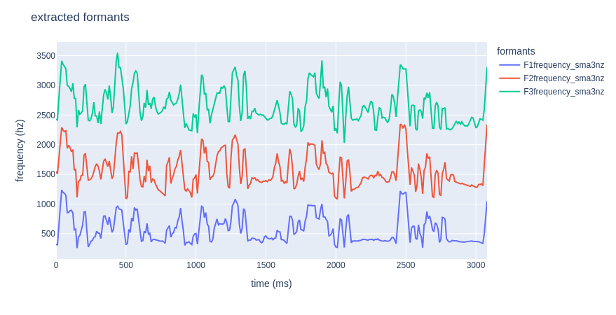
If you’d rather get a nice interactive plot, feel free to use plotly!
# import plotly!
import plotly.express as px
# plot formants
fig = px.line(formants, x="start", y=[formants['F1frequency_sma3nz'],
formants['F2frequency_sma3nz'],
formants['F3frequency_sma3nz']])
# one liner option:
# fig = px.line(formants, x="start", y=formants.columns[1:])
fig.update_layout(title="extracted formants",
	xaxis_title="time (ms)",
	yaxis_title="frequency (hz)",
	legend_title="formants")
fig.show()
bibliography
- Florian Eyben, Martin Wöllmer, Björn Schuller: “openSMILE - The Munich Versatile and Fast Open-Source Audio Feature Extractor”, Proc. ACM Multimedia (MM), ACM, Florence, Italy, ISBN 978-1-60558-933-6, pp. 1459-1462, 25.-29.10.2010.
- F. Eyben et al., “The Geneva Minimalistic Acoustic Parameter Set (GeMAPS) for Voice Research and Affective Computing,” in IEEE Transactions on Affective Computing, vol. 7, no. 2, pp. 190-202, 1 April-June 2016, doi: 10.1109/TAFFC.2015.2457417.
additional resources
- speech surfer, a great blog about speech processing technologies. They have quite a few tutorials for openSMILE! It is through one of their tutorials that I learnt how to use it! Kudos to them!!! ૮ ˶ᵔ ᵕ ᵔ˶ ა